Factorial ANOVA, Two Dependent Factors (Jump to: Lecture | Video )

The Factorial ANOVA (with two dependent factors) is most like an extension of a Repeated-Measures ANOVA.

Here's an example of a Factorial ANOVA question:

Researchers want to compare the anxiety levels of six individuals at two marital states: after then have been divorced, and then again after they have gotten married. Anxiety is measured at three times: Week 1, Week 2, and Week 3. Anxiety is rated on a scale of 1-10, with 10 being “high anxiety” and 1 being “low anxiety”. Use alpha = 0.05 to conduct your analysis.

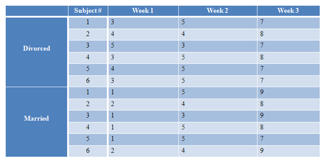
Figure 1.

Let's try a full example:

Steps for Factorial ANOVA, Two Dependent Factors
1. Define Null and Alternative Hypotheses 2. State Alpha 3. Calculate Degrees of Freedom 4. State Decision Rule 5. Calculate Test Statistic 6. State Results 7. State Conclusion

1. Define Null and Alternative Hypotheses

Here, we have three. One for each main effect, and one for the interaction.

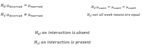
Figure 2.

2. State Alpha

alpha = 0.05

3. Calculate Degrees of Freedom

Before we start calculating our degrees of freedom, let's look at our source table:

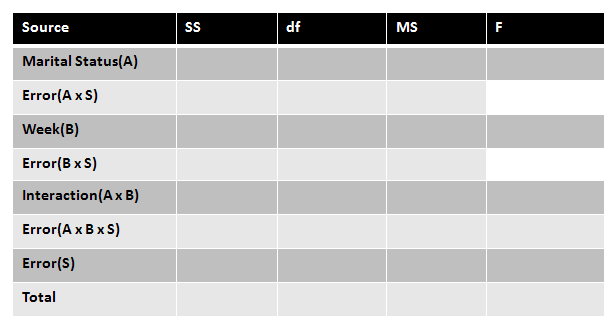
Figure 3.

Here we have 8 SS. 3 are associated with each of our effects. Each of our effects also have their own error terms. We also have a separate error term for subjects, because all of our variables are dependent. And finally, we have SS total. We will need to find all of these things to calculate our three F statistics.

Degrees of freedom are calculated as follows. "a" is the number of a groups you have, "b" is the number of b groups you have, "n" (sometimes called "s") is the total number of scores in each cell, and "N" is your total number of scores.

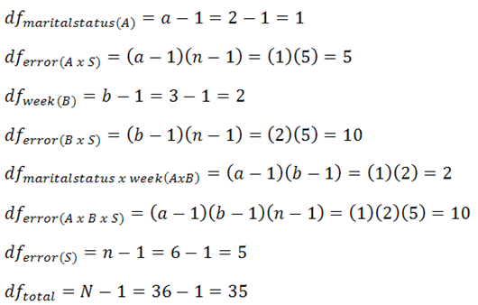
Figure 4.

4. State Decision Rule

We have three hypotheses, so we have three decision rules. Critical values are found using the effect and error degrees of freedom for our three effects:

Figure 5.

We now head to the F-table and look up our critical values using alpha = 0.05. In the table, we find the critical values shown below:

Figure 6.

These critical values bring us to our three decision rules:

[Marital Status] If F is greater than 6.61, reject the null hypothesis.

[Week] If F is greater than 4.10, reject the null hypothesis.

[Interaction] If F is greater than 4.10, reject the null hypothesis.

5. Calculate Test Statistic

First, we'll put the degrees of freedom that we've already calculated into our source table:

Figure 7.

Next, we need to find the eight SS values we are missing:

Figure 8.

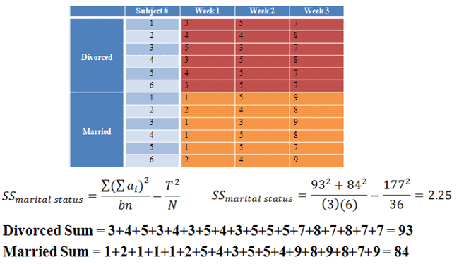
Figure 9.

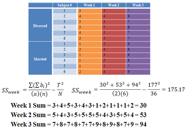
Figure 10.

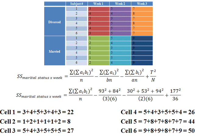
Figure 11.

Figure 12.

These SS values are then placed into our source table.

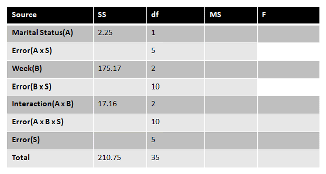
Figure 13.

Now, we start calculating our error terms.

First, A x S:

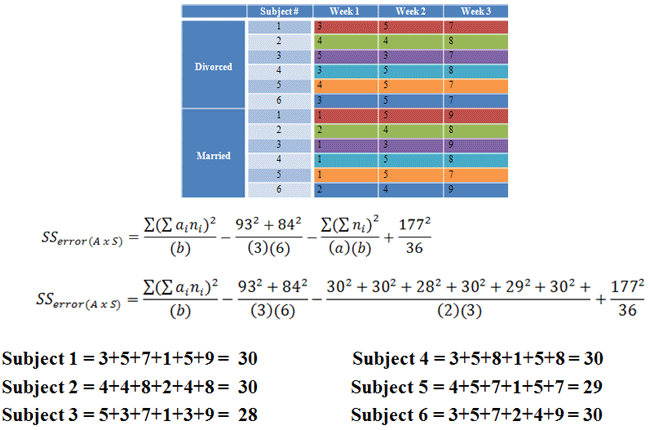
Figure 14.

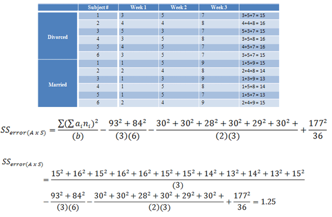
Figure 15.

Next, B x S. The first part of the B x S equation is found by summing every subjects' score at each level of "week":

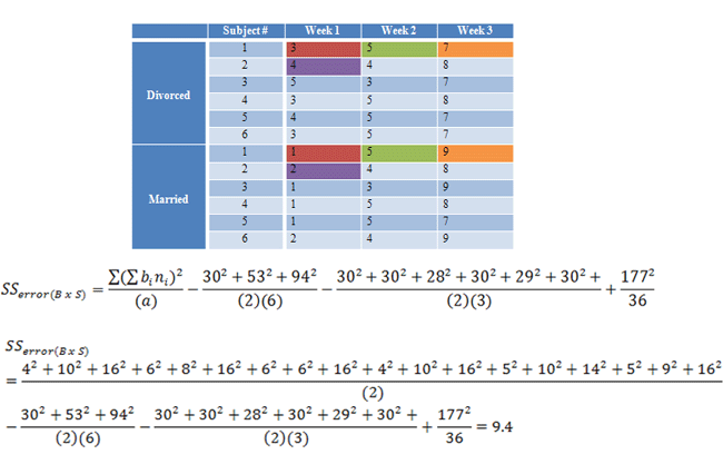
Figure 16.

And finally, S. Luckily, we've already calculated every part of it and now just need to find the final answer:

Figure 17.

We then place all of our values into the source table. We find the last missing value, A x B x S, by subtracting every value we've found from the total.

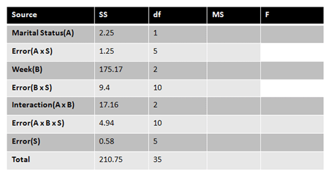
Figure 18.

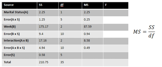
Each MS value is found by dividing each SS by their respective degrees of freedom:

Figure 19.

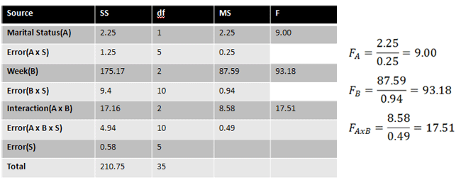
Finally, our three F values are found:

Figure 20.

6. State Results

[Marital Status] If F is greater than 6.61, reject the null hypothesis.

Our F = 9.00. Reject the null hypothesis.

[Week] If F is greater than 4.10, reject the null hypothesis.

Our F = 93.18. Reject the null hypothesis.

[Interaction] If F is greater than 4.10, reject the null hypothesis.

Our F = 17.51. Reject the null hypothesis.

7. State Conclusion

Anxiety levels differed significantly for divorced and then remarried individuals, F(1, 5) = 9.00, p < 0.05. There was a significant difference between the three different weeks, F(2, 10) = 93.18, p < 0.05. An interaction effect was also present, F(2, 10) = 17.51, p < 0.05.

---